LIWC

Compare N-gram Frequencies

A common question in corpus linguistics — and really, all kinds of text analytics — is how the language in one dataset compares to the language found in some other, comparison dataset. LIWC-22's "Compare Frequencies" feature allows you to make a statistical comparison between 2 corpora to identify what words and/or phrases (i.e., "n-grams") are most "characteristic" of each dataset.

To run the "Compare Frequencies" analysis, you will need to have 2 separate text datasets that you would like to compare. LIWC-22 will then analyze each dataset for its word/phrase frequencies. Your results, then, will be provided in 2 forms:

1. A complete table of word frequencies for both of your datasets, including statistical metrics that reflect the degree of difference (or, put another way, how "strongly" any given word/phrase is associated with one dataset versus the other);
2. Word clouds that visualize which words are more strongly associated with each corpus.

Getting Started

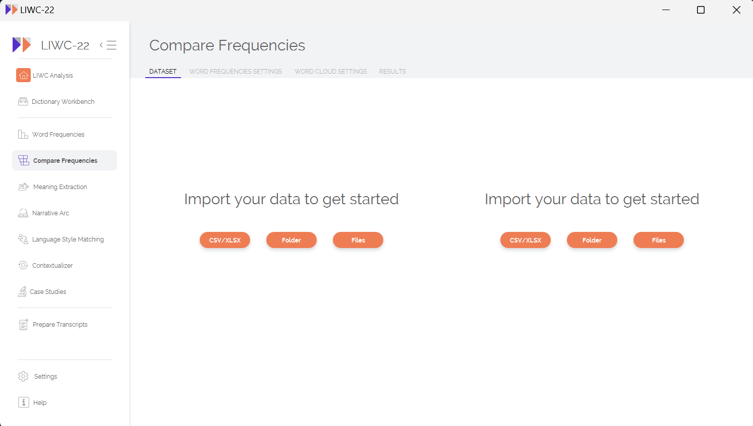
When you first choose the "Compare Frequencies" feature in LIWC-22, you will be presented with a screen that asks you to select 2 different datasets. Each dataset can be in any of the accepted formats/structures (e.g., a spreadsheet file, a folder containing various types of text documents, etc.). Note that your two datasets do not need to be in the same format; one dataset can be a CSV file, and the other a folder full of .txt files, for example.

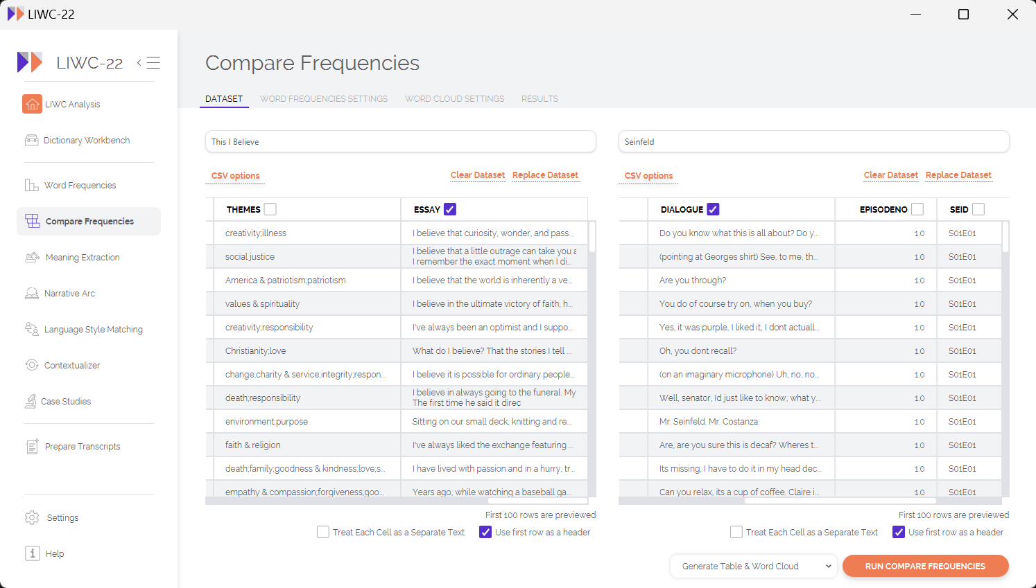
Once you have selected your 2 datasets for analysis, be sure to give them short names that will help you to identify which one is which in your results/output files. In this example, I am analyzing a dataset of people talking about what they believe to be important and comparing it against the dialogue from the hit TV show Seinfeld.

What's the deal with corpus linguistics?

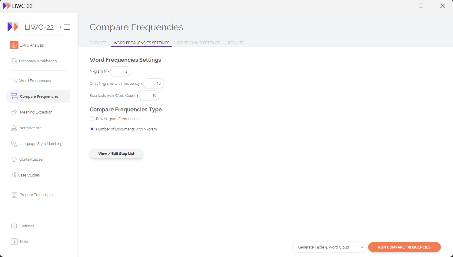
Before running your analysis, you will want to think about what values make sense for the various analysis settings that can be found under the "Word Frequencies Settings" tab. A brief description of these settings is provided below:

• N-gram N: How long would you like the phrases to be that you compare across datasets? For most people, 1-grams and 2-grams is sufficient. As you increase the value of N (e.g., 4-grams, 5-grams), you will find increasingly rare phrases that might show a strong statistical association with one dataset versus the other, but these highly specific/idiosyncratic phrases may not be meaningful for your interpretation of broad differences between the two datasets. However, you should make this decision based on your own research needs — if you are unsure, 1-grams are recommended.


• Omit N-grams with frequency <: When comparing word frequencies to get a deep sense of how two datasets differ, we typically do not learn much from words that appear only a few times across all of our data. As such, you may want to omit especially infrequent words/phrases to speed up the analysis, and to help "declutter" your results by omitting words that have a low base rate. For most social scientific use-cases, setting a value of something like 5 or 10 is sufficient, although this decision should be guided by your specific research aims and the size/diversity of your data.


• Skip texts with Word Count <: Similar to the above, we often want to skip texts that are too short to meaningfully contribute to our overall results. This setting will skip over texts that do not contain enough words to meet your needs.


• Compare Frequencies Type: When conducting statistical comparisons between your 2 datasets, there are two ways to think about the type of comparison that matters. In traditional corpus linguistics, the primary focus is often the actual appearance of each word/phrase in your data — does a word appear more frequently than you would expect by chance in one dataset versus the other? For our friends in other social sciences, however, the more meaningful unit of observation is the document itself — does a word appear more frequently at the document-level in one dataset than we would expect to be the case by chance alone? In the social sciences, "document" is often analogous to "person," which means that the question really becomes something like "Are people in this dataset more likely to use a given word/phrase than people in the other dataset?" Choosing which type of metric to use for statistical comparison is often mostly a function of which discipline you are coming from, and you should follow your intuitions about what type of comparison is the most meaningful given your own research question.


• Stop List: A "stop list" is a list of words/phrases that you want to omit from analyses. For LIWC-22, we have multiple stop list options built into the application, but you are also able to use your own, custom-made stop list as well.

For our Belief-versus-Seinfeld analysis, we will use the following settings:

Interpreting Output

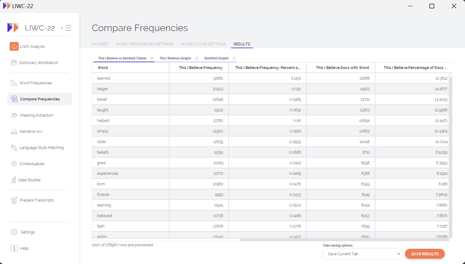
When it comes to interpreting the output from the "Compare Frequencies" analysis, there are several metrics of interest. First, in the output table itself, you will find basic descriptive statistics for each n-gram, including its frequency and the percentage of documents that contained each n-gram. Beyond this, most scholars will be interested in the comparison metrics themselves, which include:

• Log Likelihood (LL)
• %DIFF
• Bayesian Information Criterion (BIC)
• Relative Risk (RRisk)
• Odds Ratio (OR)
• Log Ratio (LR)

For the above metrics, LL and BIC can be thought of as measures of "effect size" that provide you with a statistical sense of the magnitude of difference in n-gram frequency between two corpora. The other metrics (%DIFF, RRisk, OR, LR) are various ways of characterizing the nature of such differences by showing which n-grams are more strongly associated with one corpus versus the other. LIWC-22 provides metrics for every n-gram in table format, making it relatively easy to explore which words are most strongly differentiating between your 2 datasets, as well as the directionality of differentiation.

LIWC-22 also allows you to plot word clouds for each of your 2 datasets, visualizing which words more strongly associate with one corpus or the other. In our test case, we find that words like learned, belief, and faith are most strongly associated with the "This I Believe" corpus.

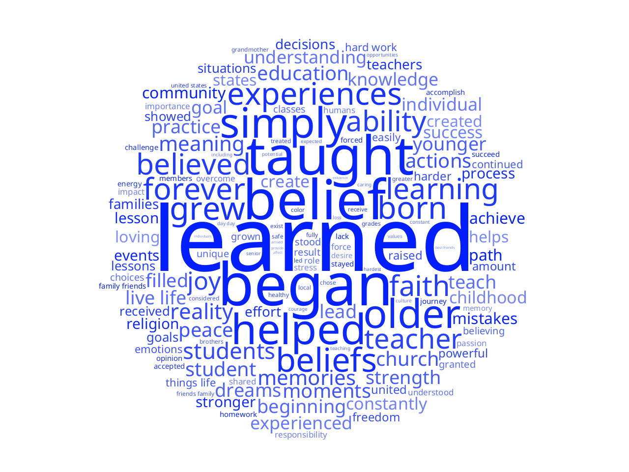
This result is intuitive — given the "no hugging, no learning" mantra of the show Seinfeld, we would expect words associated with personal beliefs and growth to be much more strongly associated with the "This I Believe" corpus. What do we see, then, when we look at the words most strongly associated with the language of Seinfeld?

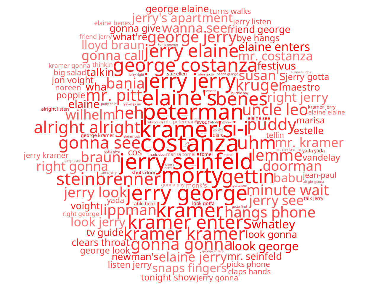
What immediately jumps out is that the Seinfeld corpus shows an disproportionate number of references to names of the show's various characters, which makes sense for 2 reasons: 1) the dataset itself is spoken dialogue rather than essays, and characters are likely to make direct references to other people within the show's universe, and 2) names like "Kramer" and "Costanza" are highly specific to the show and we would not expect to see them commonly used in long essays about personal beliefs. We also see several highly characteristic elements of the show, such as the holiday of Festivus, the word apartment (which is a common setting in the show), and much more casual language (e.g., gonna, wanna) that is consistent with spoken dialogue. Put simply, there is a lot more yada, yada, yada in the Seinfeld corpus.